Adventures in Optical Flow

Measuring Motion through Optics

I’ve been looking to add motion and velocity estimation to my 4WD IoT Robot for a while. The current motors do not have rotary encoders and there isn’t the space to install seperate ones, so I was looking for another approach. I did look at estimation through combing an IMU, Kalman Filter and GPS fixes, when I get them, but that felt like it wasn’t going to be accurate enough. Therefore, I started to look at Optical Flow Sensing.

Optical Flow - How does is work?

Optical flow sensors work by sampling images from a digital camera at some specified frame rate and detecting the movement by changes in the pixels. Optical flow sensors have been around a while and are the basis of an optical mouse. However, the class of device you find in an optical mouse do not have the focal length, field of view (FoV) and other optical properties for them to be suitable for robotics applications. The diagram below (courtesy of Nanonets.com) outlines the theory. 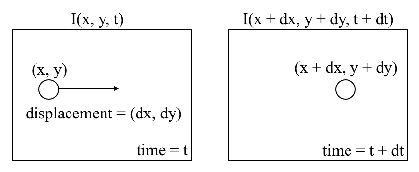if you express the image I as a function of space (x,y) and time (t) such that you take the first image I(x,y,t) and move the pixels by (dx,dy) over time (t) you obtain a new image that can be expressed as I(x+dx,y+dy,t+dt). Taking the Taylor Series Approximation then dividing by dt you arrive at the optical flow equation shown below.

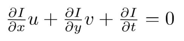
This is where u=dx/dt and v=dy/dt and dI/dx,dI/dy and dI/dt are the image gradients across the horizontal, vertical and time dimensions. This equation cannot be directly solved for u and v as there are two unknown variables. This is resolved using a method called Lucas-Kanade that makes assumptions around image movement being in small increments and weights can be applied to the moving image window.

So, show me the sensor

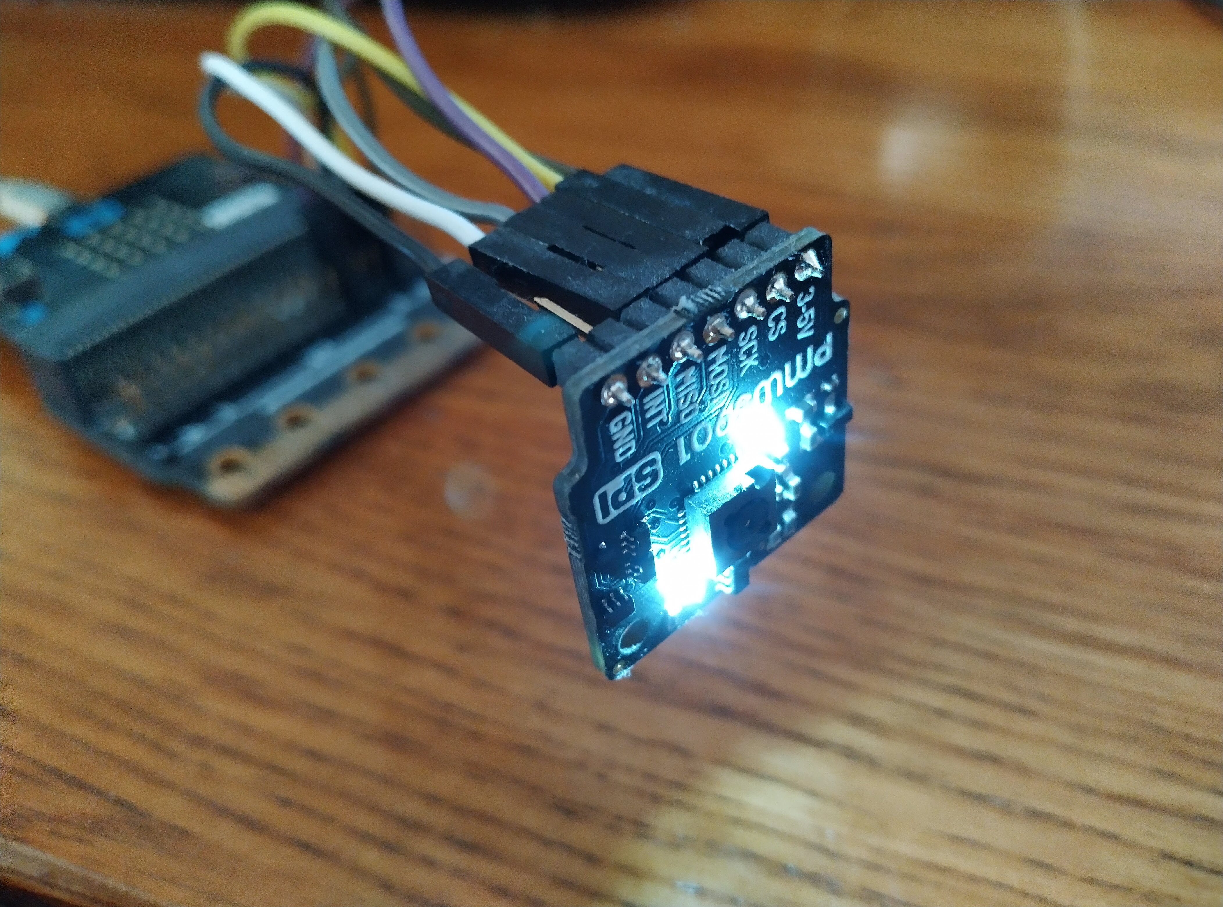
There are a number of reasonable cost optical flow sensors on the market. However, a number of them use the common optical image system found in optical mice and, as mentioned previously, do not provide the FoV and focal length required. For example, if you lift you optical mouse off a surface just by a very tiny fraction it’s likely to stop working. Therefore the sensor I chose is the Pixel Art PMW3901MB-TXQT. A picture of the core sensor module is shown below.

This device has a focal range of a minimum of 80mm to infinity with a FoV of 42 degrees, a 121 FPS framerate at a maximum rate of 7.4 radians per second. This is packaged up into the PCB you see in the photo at the start of this article. As you probably appreciate, the calculations involved in optical flow are quite intensive and would place considerable load on the low power microcontrollers. Therefore the pmw3901mb-txqt has a dedicated motion processor that peforms these calculations in hardware. Connectivity to a microcontroller is via SPI.

So how do you get data off it?

Those of you with a keen eye (and knowledge of microcontroller platforms) will of spotted a BBC MicroBit in the photo. Not another micocontroller I here you say. Well the problem is both the Uno and the STM32 board already have their SPI buses connected leaving the only potential option of creating a software defined SPI bus. However, I knew that a software defined SPI was just not going to be perfomant, even running on the STM32F407. Also, the MicroBit has an inbuilt LSM303AGR accelerometer and magnetometer, as well as the nRF52 Application Processor which will come in handy for the Robot anyway.

Show me the code

The first problem I encountered is I couldn’t find an existing driver for the PMW3901MB-TXQT on either the MicroBit specifically or even the nRF52 (seems to be a common theme with my projects). First job, therefore, was to get one working. Unfortunately, like a lot of these specialist devices, the datasheet is pretty sparse and appears to omit numerous bits of detail and “gotchas”.

First thing’s first, I needed a couple of wrapper functions to read and write to the SPI bus.

static SPI spi(MOSI,MISO,SCK);              //mosi, miso, sclk                
static DigitalOut cs(p16);                  //chip select on Pin p16

uint8_t readRegister(uint8_t addr)
{
    cs = 0;                                 //Set chip select low/active
    addr = addr & 0x7F;                     //Set MSB to 0 to indicate read operation
    spi.write(addr);                        //Write the given address
    wait_us(35);                            //Add a tiny delay after sending address for some internal cycle timing.
    uint8_t data_read = spi.write(0x00);    //Throw dummy byte after sending address to receieve data
    cs = 1;                                 //Set chip select back to high/inactive
    return data_read;                       //Returns 8-bit data from register
}
 
void writeRegister(uint8_t addr, uint8_t data)
{
    cs = 0;                                 //Set chip select low/active
    addr = addr | 0x80;                     //Set MSB to 1 to indicate write operation
    spi.write(addr);                        //Write the given address
    spi.write(data);                        //Write the given data
    cs = 1;                                 //Set chip select back to high/inactive
}

First step is to check the sensor is on the SPI bus by checking for 0x49h at register 0x00h.

if(readRegister(0x00) != 0x49)
{
    serial.printf("Communication protocol error! Terminating program.\n\r");
    return 0;
}

There is a whole, quite complex, sensor initialisation sequence required by the datasheet. Unfortunately there’s no real explaination of what is going on here. Most the of the intialisation is writing a sequence of codes to registers. One aspect I had to “play around” with and discover was switching on the LEDs to aid with low light scenarios. You can see the LEDs on in the photo.

writeRegister(0x7f, 0x14);              // Turn on LEDs
writeRegister(0x6f, 0x1c);
writeRegister(0x7f, 0x00);

Now we can get some data!

// Check for motion
if(readRegister(0x02) & 0x80) {
    deltaX_low = readRegister(0x03);                //Grabs data from the proper registers.
    deltaX_high = (readRegister(0x04)<<8) & 0xFF00; //Grabs data and shifts it to make space to be combined with lower bits.
    deltaY_low = readRegister(0x05);
    deltaY_high = (readRegister(0x06)<<8) & 0xFF00;
        
    deltaX = deltaX_high | deltaX_low;              //Combines the low and high bits.
    deltaY = deltaY_high | deltaY_low;
}

Now the deltaX and deltaY values are relative pixel movements. To translate these into some useful units of measure you need the following calculation.

distance = (sensor_reading x distance_to_image / sensor_resolution ) x 2 x tan(field_of_view / 2.0)

Where distance_to_image is distance from the sensor to the image. In my application, with a minimal focal length of 80mm, I have the sensor pointing up to my ceiling which is ~2.4m. The sensor field of view is 42 Degress and the resolution is 30x30 pixels.

So is it accurate?

I’ve done some bench testing with not too bad results. I’ve yet to get the system installed on the Robot as I need to design and 3D print some fixings for it. With the Robot currently having a GPS I should be able to combine GPS and Optical Flow with a Kalman Filter estimator to get the best motion and velocity estimation possible.

Can you create your own Optical Flow sensor?

The answer is yes. Any digital video camera can be used to measure optical flow. There’s a great tutorial using OpenCV that should work with any camera system / sensor. Obviously the higher the image resolution and looking to deal with optical flow in 3D is substantially more computationally expensive that what the sensor here does. There are projects out there that have successfully got 3D optical flow running on a Raspberry Pi 2, though I suspect not leaving much CPU headroom for other tasks.