Explaining AI - From First Principles with Python
As we all know, AI is everywhere. However I’ve been increasingly concerned that the field is not very widely understood and is subject to considerable levels of misunderstanding. I think the Tech industry, consultancies and vendors don’t help here with all the buzz and hype.
So, I’ve started a series of looking at the fundementals of AI, specifically the underpinning mathematics and algorithms. Providing the history and development of particular techniques, such as Deep Learning, and providing an implementation from first principles in the Python programming language.
First in this series is looking at the Perceptron. The basic component that underpins all classes of Neural Networks, including Deep Learning.
Biological Neurons
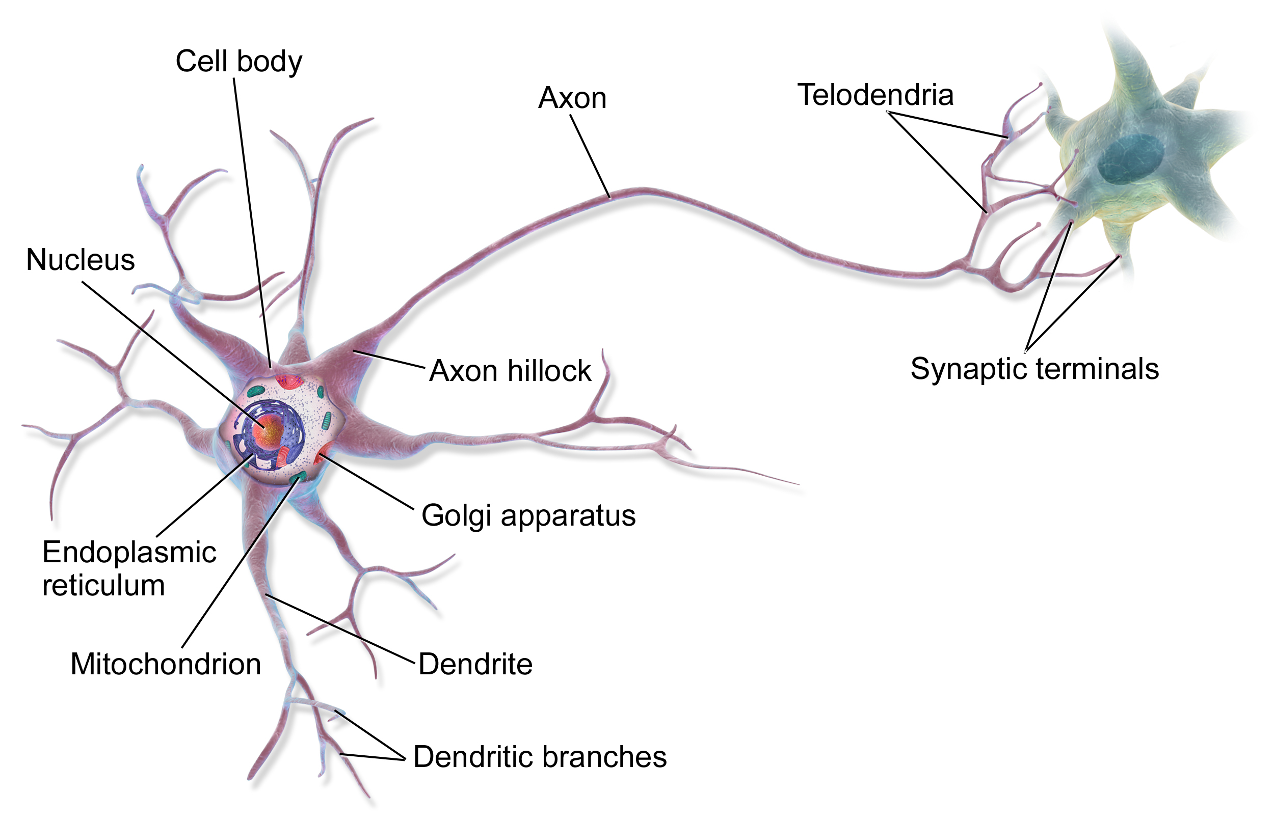
I’m not planning to go in-depth on the biological neuron, but it’s key to understanding where Neural Networks have come from to have a basic appreciation of a neuron.
The concept of a neuron was first proposed in the mid 19th century by a number of scientists. However, the major breakthrough came in 1891 by the German sciemtist Wilhelm Waldeyer. For a good entry introduction to Neurons I recommend this article on Khanacademy. It was understood early on that Neurons are the information processing backbone of biological systems. Essentially, a neuron has three basic functions:
- Receive signals (information)
- Integrate these received signals and determine what information should be passed on
- Send the integrated and procesed information on as signals to connected neurons
Artificial Neurons
It will be obvious to any Computer Scientist or Software Engineer that the description of a biological neuron is analogeous to a generalised information processing function.
In the 1940’s, this analogy is exactly what Warren McCullock and Walter Pitts outlined their seminal paper A Logical Calculus of the Ideas Immanent in Nervous Activity. This paper is the foundation for all the work in Neural Networks and Deep Learning that has been developed since.
An Artificial Neuron can be simply stated as a mathematical function that takes a series of inputs, computes a function on these inputs that generates an output.
Perceptron
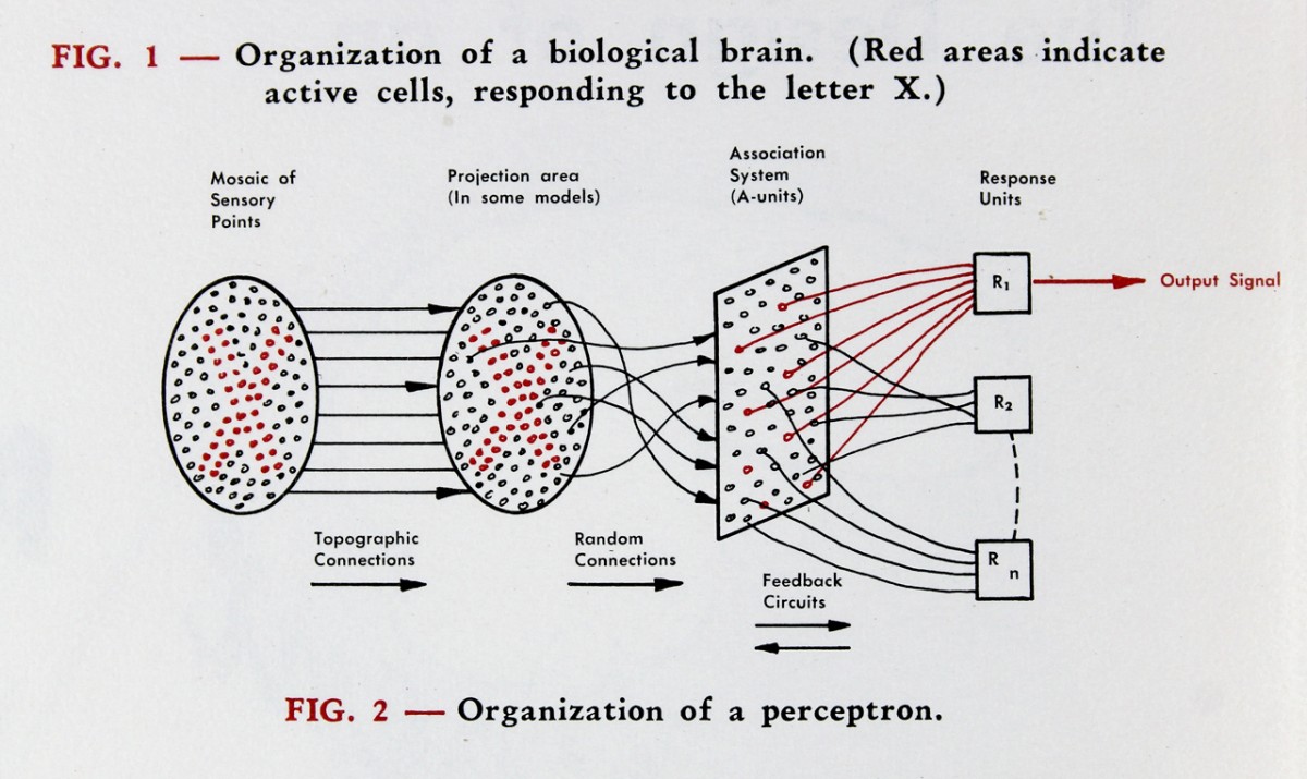
McCullock and Pitts work was further developed in the 1950s by Frank Rosenblatt who was a Research Psychologist and Project Engineer at the Cornell Aeronautical Laboratory. Rosenblatts work culmulated in the first Neural Network implementation on an IBM 704. Rosenblatt described his system Perceptron. You can read his 1958 paper here.
The figure below is from Rosenblatt’s original paper showing the architecture of a Percepton.
 A modern simplified version of Rosenblatt’s diagram is shown below.
 Probably the most important element on this diagram is the Activation Function. This is a function that causes the Neuron to “fire” and send an output. Complex multilayered Neural Networks can use many different activiation functions, but the most simplest is what’s called the Step Function shown below.
 The Step Function activates, or “fires”, when the input sum function is greater than a threshold value. In this case between 0 and 1.
The Perceptron Algorithm
The core algorithm for a perceptron goes like this:
Given a input of a vector X with a matching target classification vector y
Given a learning rate (or step rate) and number of iterations
Given a provided activation function (in our case the step function)
Given a provided transfer function (in our case linear)
Given an initial set of weights of bias of the perceptron
    For each iteration
        For each dataset in vector X
            Calculate the transfer function as a dot product of the current weights plus the bias
            Get a current prediction of y from the perceptron
            Update the weights and bias as the learning rate x the actual value y versus the prediction of y
And that is it, the basic algorithm for the simplest Neural Network a single Perceptron. This basic Perceptron does have limitations in that it can only cope with a two state classification problem and where the two datasets can be seperated linearly.
Show me the Code
Here’s the walkthrough in Python. I’ve attempted to keep the code as close to core Python as possible, but I’ve leveraged Numpy to simplify vector computation (e.g. calculating the dot product) and Scikit-Learn to aid the generation of a sample dataset and train / test split.
First, lets import some Python libraries
import numpy as np
from sklearn.model_selection import train_test_split
from sklearn import datasets
import matplotlib.pyplot as plt
Now lets generate a sample dataset of 150 samples with two features, two centres (for the clusters) using a standard deviation of 1.05
X, y = datasets.make_blobs(n_samples=150,n_features=2,centers=2,cluster_std=1.05,random_state=2)
Here’s what X looks like.
array([[ -0.53278301,  -1.64847081],
       [ -0.55022637, -11.61661524],
       [  1.38862276,  -1.4358059 ],
       [  1.37033956,  -0.64022071],
       [ -0.88060639,  -9.7094674 ]])
and y
array([1, 0, 1, 1, 0])
Here’s all the values of X plotted as a scatter.
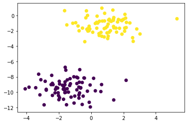
Visually, you can clearly see that the dataset X splits into two distinct clusters. In an image recognition algorithm this dataset could represent pixels from images of cats and dogs. For example, in the target classification dataset y 0 could be cat and 1 dog.
So lets code the actual Perceptron. First lets set the weights and bias to 0. In some implementations you may decide to set these with a level of random values.
self.weights = np.zeros(n_features)
self.bias = 0
Next set _y to the target classification set, ensuring that we only have a two state classification of 0 or 1.
y_ = np.array([1 if i > 0 else 0 for i in y])
Now the here’s the learning part.
for _ in range(self.n_iters):
    for idx, x_i in enumerate(X):
        transfer_func = np.dot(x_i, self.weights) + self.bias
        y_predicted = self.activation_func(transfer_func)
        # Perceptron update rule
        update = self.lr * (y_[idx] - y_predicted)
        self.weights += update * x_i
        self.bias += update
The code above demonstrates why Neural Networks, and Deep Learning in particular, are so computational expensive. As you can see the outer loop runs a number of learning / training iterations (or epochs) and for each one of those the transfer, activation functions and update calculations need to be computed. Bear in mind this is a single Perceptron, not actually a Neural Network. As of time of writing, the biggest Deep Learning network out there is Microsoft Turing NLG with over 17 billion parameters and a network with 78 layers with a hidden layer of 4256 perceptrons.
Once the model is trained, running predictions is substantially less computationally expensive. What’s happening here is that the activation function, which can only return possible classifications of 0 or 1 is being computed by returning the value at the weight and bias ‘position’ in the model.
def predict(self, X):
    transfer_func = np.dot(X, self.weights) + self.bias
    y_predicted = self.activation_func(transfer_func)
    return y_predicted
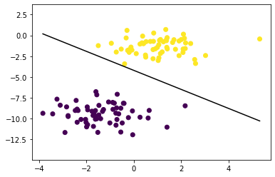
By accessing the weights and bias of the model at the min and max of the training set and knowning our transfer function is linear, we can extract the ‘line’ that shows how the Perceptron has seperated the two classifications.
X_train, X_test, y_train, y_test = train_test_split(X, y, test_size=0.2, random_state=123)
p = Perceptron(learning_rate=0.01, n_iters=1000)
p.fit(X_train, y_train)
predictions = p.predict(X_test)

print("Perceptron classification accuracy", accuracy(y_test, predictions))

fig = plt.figure()
ax = fig.add_subplot(1,1,1)
plt.scatter(X_train[:,0], X_train[:,1],marker='o',c=y_train)

x0_1 = np.amin(X_train[:,0])
x0_2 = np.amax(X_train[:,0])

x1_1 = (-p.weights[0] * x0_1 - p.bias) / p.weights[1]
x1_2 = (-p.weights[0] * x0_2 - p.bias) / p.weights[1]

ax.plot([x0_1, x0_2],[x1_1, x1_2], 'k')

ymin = np.amin(X_train[:,1])
ymax = np.amax(X_train[:,1])
ax.set_ylim([ymin-3,ymax+3])

plt.show()
And here’s the scatter plot again, with the classification boundary extracted from our Perceptron model.
So that’s it, the simplest implementaton of a ‘Deep Learning’ model. The Jupyter Notebbok for this can be found in my Github repo.
Hope you’ve find this useful and, more importantly, helped demistify Neural Networks and Deep Learning.